Word Embeddings
🧠 Word Embeddings: The Evolution of Machine Understanding
Imagine trying to teach a computer to read. For us, words are rich with meaning, nuance, and history. But for a computer, they are just strings of characters. How do we bridge this gap? How do we turn the poetry of language into the cold logic of mathematics?
This is the story of Word Embeddings—the journey of teaching machines to understand not just words, but meaning.
📌 The Problem: When Words Were Just Numbers
In the early days of Natural Language Processing (NLP), we treated words like distinct islands. We used techniques like One-Hot Encoding, where every word in the dictionary was assigned a unique index.
Imagine a vocabulary of 10,000 words. In this system:
- “Apple” might be
[1, 0, 0, ..., 0] - “Orange” might be
[0, 1, 0, ..., 0]
While simple, this approach had a fatal flaw: Orthogonality. Mathematically, the dot product of these two vectors is zero. To the computer, “Apple” and “Orange” are as unrelated as “Apple” and “Bicycle”. There is no shared meaning, no semantic connection.
Furthermore, this method suffered from the Curse of Dimensionality. As your vocabulary grew to millions of words, your vectors became impossibly large and sparse (mostly zeros), making computation inefficient. We needed a way to capture the soul of the language—a way to represent words so that similar concepts lived close together in a dense mathematical space.
This need drove the four main goals of modern embeddings:
- Dimensionality Reduction: Turning massive, sparse vectors into compact, dense ones (e.g., 300 dimensions instead of 100,000).
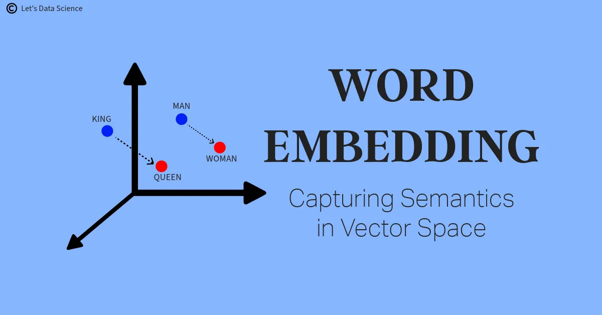
- Semantic Similarity: Teaching the model that King is to Queen what Man is to Woman.
- Shared Spaces: Allowing recommendation systems to map users and items in the same universe.
- Transfer Learning: Letting models learn from vast amounts of text once, then apply that knowledge everywhere.
A Brief History of Meaning
The evolution of text embeddings is a timeline of increasing complexity and understanding. We moved from simple counting (how many times does this word appear?) to static vectors, and finally to the dynamic, context-aware models we use today.
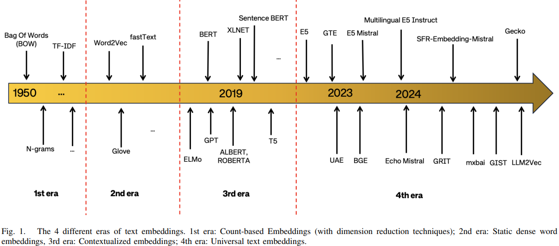
A timeline illustration showing the evolution of word embedding models, from early one-hot and count-based representations to modern neural embeddings and contextual models.
⚙️ The Second Era: Words Find Their Place (Word2Vec)
The real breakthrough came when we stopped counting words and started looking at their neighbors. The idea was simple but profound: “You shall know a word by the company it keeps.” (J.R. Firth, 1957).
This gave birth to Word2Vec. The genius of Word2Vec wasn’t that it was a deep neural network (it’s actually quite shallow), but that it used a “Fake Task” to learn.
We didn’t actually care about the model’s prediction accuracy. We trained a neural network to predict a word from its context (or vice versa), but we threw away the predictions. What we kept were the weights of the hidden layer. These weights became the word embeddings.
| Model | The Narrative | Direction |
|---|---|---|
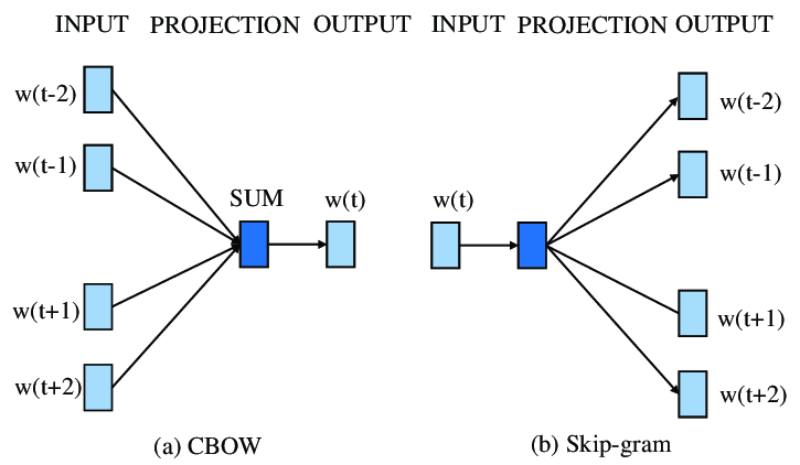
| CBOW (Continuous Bag of Words) | “I see the context (‘the’, ‘cat’, ‘on’, ‘mat’), can I guess the missing word (‘sat’)?” | Context → Target |
| Skip-Gram | “I see the word (‘sat’), can I guess the context (‘the’, ‘cat’, ‘on’, ‘mat’)?” | Target → Context |
For the first time, words weren’t just indices; they were vectors in a high-dimensional space. The model learned that “King” and “Man” share a direction, and “Queen” and “Woman” share that same direction.
This allowed for vector arithmetic: \(\text{Vector("King")} - \text{Vector("Man")} + \text{Vector("Woman")} \approx \text{Vector("Queen")}\)
The machine had learned an analogy.
🧩 The Third Era: The Context Conundrum
But static embeddings like Word2Vec had a limitation. They assumed a word always meant the same thing.
Consider the word “bass”:
- “He played the bass guitar during the concert.” (Musical instrument)
- “The bass swam quickly through the water.” (Fish)
To Word2Vec, “bass” was just one vector. It was a confused mix of a guitar and a fish.
This led to the third era: Deep Contextualized Embeddings. We realized that a word’s meaning is fluid—it changes based on the sentence it lives in. We needed dynamic embeddings, where the vector for “bass” shifts depending on whether it’s near “guitar” or “swam”.
The Struggle with Memory (RNNs & LSTMs)
Before Transformers, we tried to solve this with Recurrent Neural Networks (RNNs) and LSTMs. These models read text sequentially, like humans do—left to right. They tried to carry the “memory” of the sentence as they moved along.
However, they suffered from a “short-term memory” problem. By the time the model reached the end of a long paragraph, it often forgot the beginning. They couldn’t effectively connect a word at the start of a sentence to a word at the end.
🧠 The Transformer Revolution
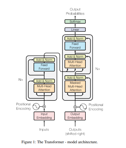
The solution came in 2017 with the paper “Attention Is All You Need”, which introduced the Transformer architecture.
Transformers changed everything by asking: “Why read left-to-right at all?”
Instead of processing words sequentially, Transformers look at the entire sentence at once. They use a mechanism called Self-Attention to allow every word to “talk” to every other word, regardless of how far apart they are. This parallelism not only solved the memory problem but also allowed for massive speedups in training.
Key Concepts
- Context Vector: A representation of meaning that evolves as the model reads.
- Positional Embeddings: Since Transformers process words in parallel (simultaneously), they have no inherent sense of order. We must inject “tags” to tell the model that “Man bites Dog” is different from “Dog bites Man”.
- Cross Attention: The bridge that allows information to flow between different sequences (e.g., from an English sentence to a French translation).
🎯 Attention Mechanisms: The Heart of Modern NLP
If the Transformer is the body, the Attention Mechanism is the soul. It allows the model to focus on what matters.
Think about how you understand the sentence: “The animal didn’t cross the street because it was too tired.” When you read “it”, your brain instantly links it to “animal”, not “street”. That is attention.
The Math Behind the Magic: A Digital Filing System
The attention mechanism is often explained using a database or filing system analogy. Imagine you are in a library:
- Query (Q): What you are looking for (e.g., “books about space”).
- Key (K): The label on the book spine (e.g., “Astronomy”, “Cooking”, “History”).
- Value (V): The actual content inside the book.
The model calculates a similarity score (dot product) between your Query and all the Keys. If the match is strong (high score), the model retrieves more of the Value.
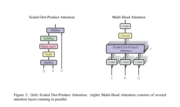
\[\text{Attention}(Q, K, V) = \text{softmax}\left(\frac{QK^T}{\sqrt{d_k}}\right)V\]The softmax ensures all the attention scores add up to 1 (100% focus distributed across words).
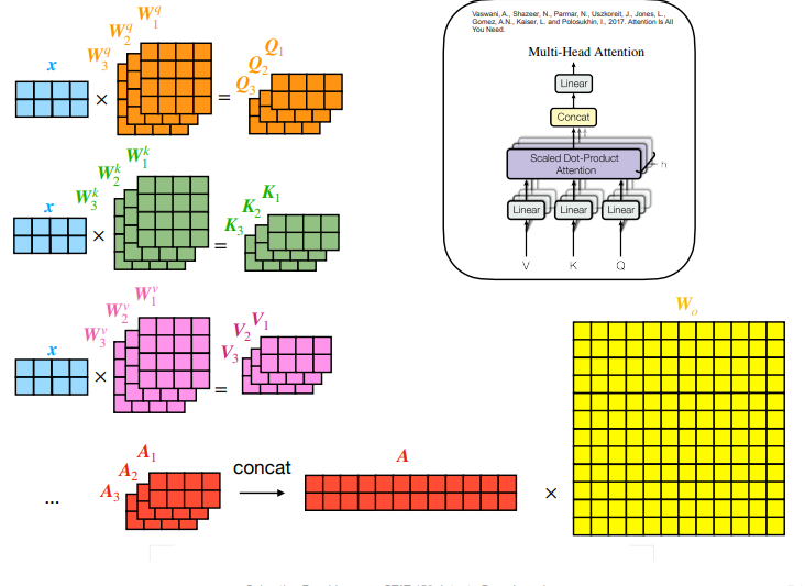
Multi-Head Attention: Seeing from All Angles
Why settle for one perspective? Multi-Head Attention allows the model to run several attention mechanisms in parallel. One head might focus on grammar, another on vocabulary, and another on long-distance relationships between words.
Seeing Attention in Action
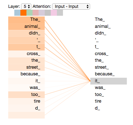
In this visualization, you can see the model “thinking.” The lines show the word “it_” attending strongly to itself and the context around it, resolving the ambiguity of pronouns just like a human reader would.
🤖 BERT: The Master of Context
The culmination of this journey (so far) is BERT (Bidirectional Encoder Representations from Transformers).
Before BERT, models like GPT (Generative Pre-trained Transformer) were Unidirectional—they read left-to-right to predict the next word. This is great for writing text, but not ideal for understanding it.
BERT changed the game by being deeply Bidirectional. It uses a “Masked Language Model” (MLM) task—essentially a “fill-in-the-blank” test.
- Input: “The [MASK] sat on the mat.”
- Task: Guess the hidden word.
To solve this, BERT must look at both the left (“The”) and the right (“sat on the mat”) context simultaneously. With 12 layers and 12 attention heads (in the Base model), it creates a deeply rich, nuanced understanding of language that previous models could only dream of.
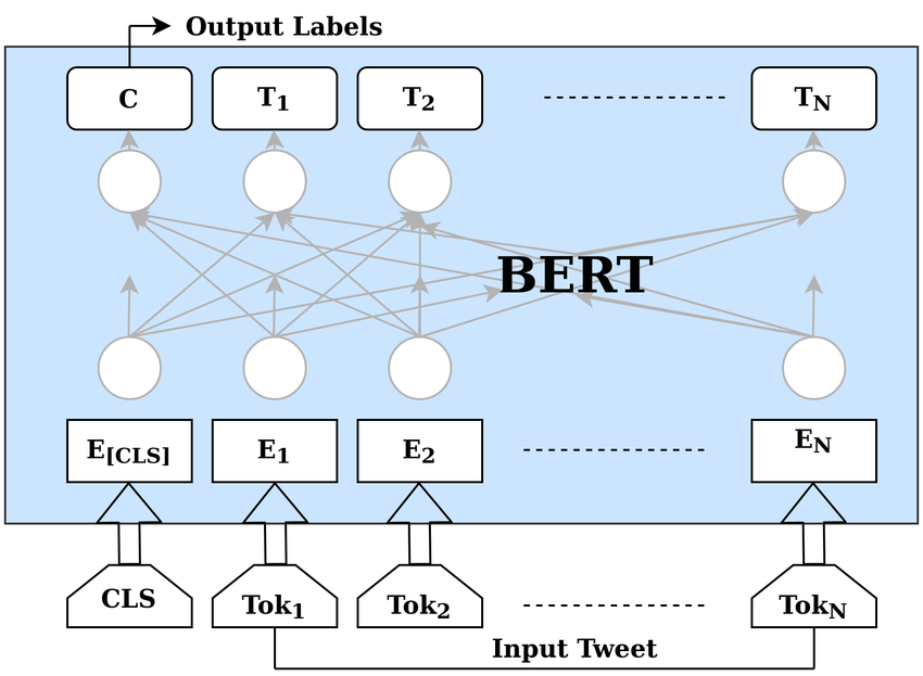
BERT processes tokens in parallel, allowing every word to “see” every other word. The [CLS] token aggregates the entire sentence’s meaning, becoming a powerful tool for classification tasks.
📊 The Road Ahead
We have come a long way from simple word counts. Today, we evaluate our models on massive benchmarks like MTEB, pushing the boundaries of what machines can understand.
As we move into the fourth era of universal text embeddings, the line between human and machine understanding continues to blur.
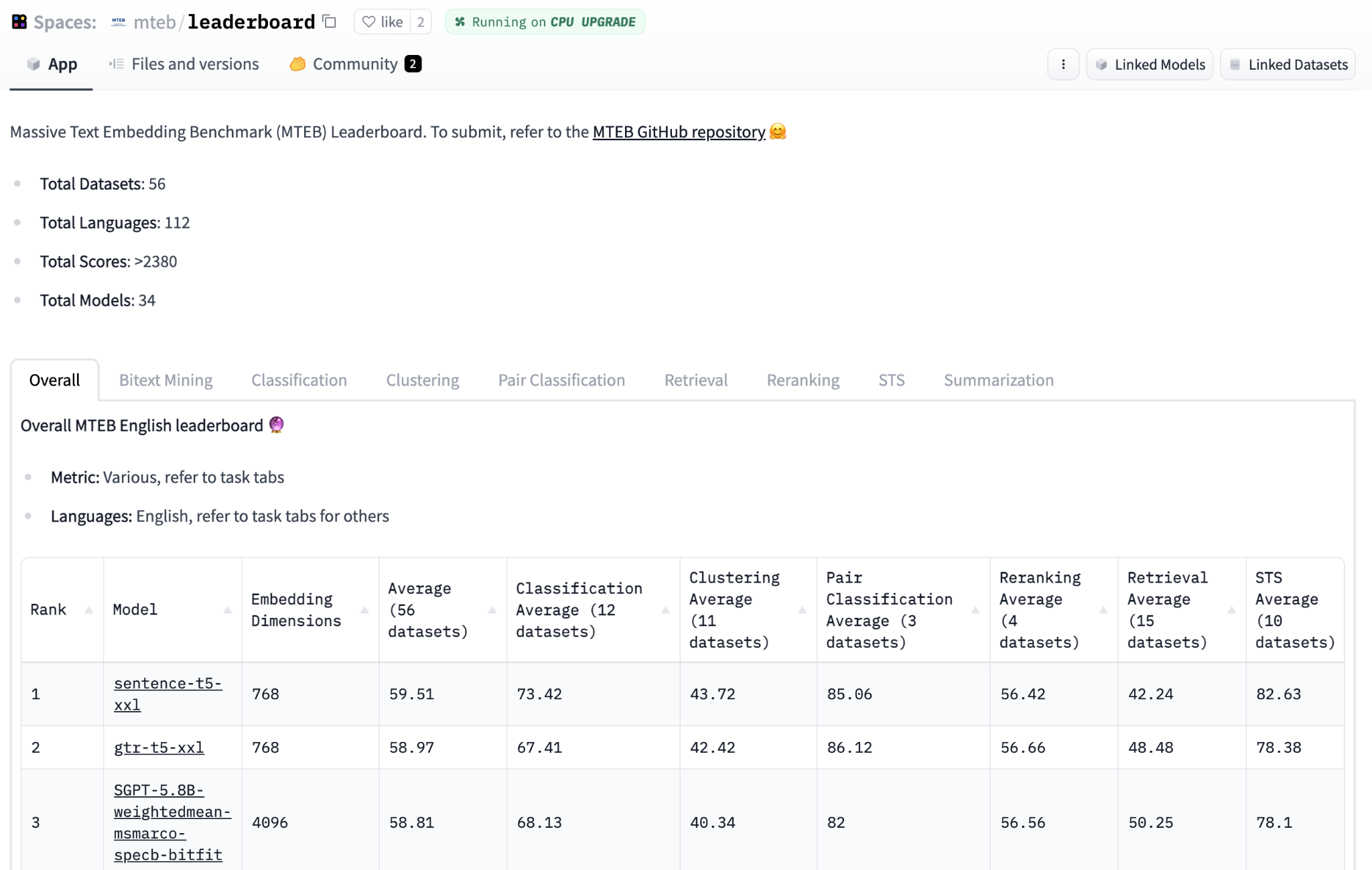
Benchmarks like MTEB allow us to evaluate models across diverse tasks such as retrieval, clustering, and semantic similarity. You can even filter for specific languages like Persian to find the best models for your needs.
📚 References
- Efficient Estimation of Word Representations in Vector Space
- Distributed Representations of Words and Phrases and their Compositionality
- Attention Is All You Need
- BERT: Pre-training of Deep Bidirectional Transformers for Language Understanding
- Recent Advances in Universal Text Embeddings: A Comprehensive Review of Top-Performing Methods on the MTEB Benchmark
- L19_seq2seq_rnn-transformers__slides